The year was 2013, I had just started my studies towards my doctorate degree and had come across Gaussian Mixture Models. I was having quite a hard time understanding and spent many hours trying to perfect what I look back to as my “Hello World” code for Gaussians Mixture Models. Little did I knew how significant these models were. Back then I could not really appreciate the beauty of what looked like a bunch of dense math equations.
Fast forward to present day, and I have grown to appreciate how fascinating those equations are, what they mean, and how almost every dataset has an embedded Gaussian somewhere. For this reason, today I am starting a series of blog posts that will be dedicated to appreciating how significant Gaussians are.
What is a Gaussian?
A Gaussian function is a mathematical function named after the mathematician Carl Friedrich Gauss. It has a unique “bell curve” shape and is widely used to represent probability density functions, sometimes also referred to as normal distribution. The simplest form of a Gaussian function is given for one-dimensional case as:
\[g(x) = \frac{1}{\sigma\sqrt{2\pi}} e^{-\frac{1}{2}\big[\frac{(x-\mu)^2}{\sigma^2}\big]},\]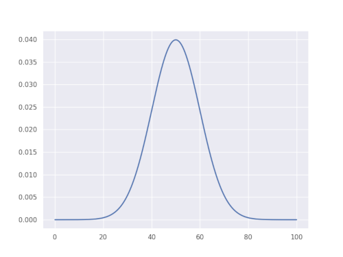
where \(\mu\) is the mean and \(\sigma\) is the standard deviation of the distribution. This means that given some empirical data, a simple Gaussian distribution can be represented as mean \(\mu\) and standard deviation \(\sigma\) of the data. It is this simple application and the fact that the function can fit many natural datasets that makes Gaussians so powerful in many fields.
|
|
Why Gaussians?
Recently I stumbled upon the BBC series called The Code, which talks about how mathematics appears in many natural phenomenon. I found myself completely fascinated by a real-life application of a Gaussian distribution presented in this show. The presenter, who himself was a mathematician, went to see a fisherman to ask some questions and collect information about his daily catch. He then took all of the fisherman’s catch for that day, which comprised around 200 fishes, and weighed each one of the fishes. He proceeded to estimate mean and standard deviation to get an estimate of a Gaussian distribution. Using the distribution the presenter estimated the weight of the biggest fish that the fisherman would have ever caught to be around 1kg. I was totally amazed to see that upon enquiring, the fisherman recalled his biggest catch to be exactly what had come out of the presenter’s Gaussian distribution. I was left amazed but also curious to know what other places could we see Gaussians in?
The idea of a Gaussian (aka normal) distribution stems from the central limit theorem which states that in some situations when independent random variables are observed (or sampled), their normalised histogram tends towards a Gaussian distribution. In other words, when randomly sampling or observing a certain quantity, the distribution of the samples tends to reach a Gaussian distribution with increased samples observed.
Gaussians in observing nature
Some examples of observations that follow a normal distribution are:
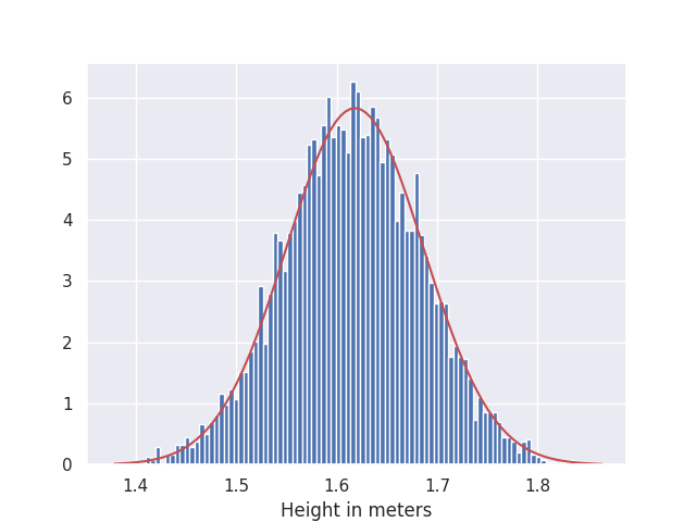
Height/weight distribution of a population: If we look at the distribution of height/weight of a population, we encounter a Gaussian distribution with mean of the distribution indicating overall average quantity, while the spread covers the range of deviation from the mean. What this implies is that if you choose a person randomly, they are more likely to have a height/weight closer to the mean of the population, since the probability for these is much greater. Similar to the presenters’ example above, we can estimate the tallest/shortest height or heaviest/lightest weight person that could be found within the population. In the following figures, a histogram of height/weight is visualised and compared against a Gaussian distribution (in red) for dataset from kaggle.
|

|
Distribution of weather data: For a given geographical location, temperatures/rainfall in a specific season can also be easily modelled with a Gaussian distribution. It also provides interesting insights about maximum/minimum expected rainfall/temperatures.
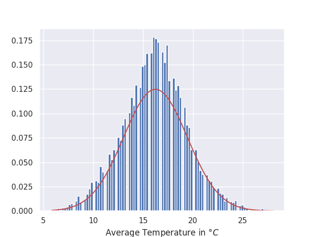
As an example, I took past 20 years of average temperatures for summer season for London, UK and plotted their histogram against a Gaussian distribution fitted on the same data (it is quite close to a Gaussian but not a perfect fit):
Other examples There are many other natural events/datasets that follow a Gaussian distribution, e.g. clinical data related to a disease/diagnosis, blood pressure, heart rate, IQ of a population, measurement error, manufacturing errors etc etc. In fact, if you have a google maps application on your phone, then you should be able to check how busy your favourite store would be tomorrow at 5pm and also how much time a typical customer spends there, thanks to Gaussians!

Disclaimer - not all phenomenon follow normal distribution: Just a disclaimer for the readers, while Gaussians can be used in modelling many datasets, they certainly don’t apply to everything. There are many discussions on this, a good one can be found here.
Gaussians in data-driven machine learning
In recent years, significant advancements have been made in data-driven machine learning field. While this is widely attributed to the innovative research from many amazing researchers, there are two main contributing factors that led to enabling these advancements. First, processing power, especially the use of GPUs, has exponentially grown to accelerate processing and learning from very large datasets. Secondly, and most importantly, the age of information has enabled collection of colossal amounts of data. It is estimated that each day 300 hours of videos are uploaded on youtube, and over 95 million images are uploaded to instagram alone.
Since data-driven machine learning relies on data collection, it is important to understand the sources of variations within the associated datasets. These could be ranging from actual variations in the data, such as pictures of different kinds of cats, as well as variations due to noisy collection/labelling process. Moreover, while we can collect huge amounts of data, we are still able to label and use a finite set, which can only be used to model a subset of the underlying reality resulting in noisy models. As I will demonstrate through the example in the next section, in most cases these variations follow the central limit theorem and hence can be modelled using Gaussians.
Simulating errors in data collection
A long time back, I got introduced to Monte-Carlo methods with an experiment that looked at estimating the value of \(\pi\) using only simulation of the sampling method. The idea was to estimate the value of \(\pi\) using the equations of circle and area.
The circle equation defines a circle with radius \(r\) as:
\[r^2 = x^2 + y^2\]Looking at the area of square with side length \(2r\) and comparing against area of a circle with radius \(r\) (as shown in the following figure), we get the following ratios:
\[\frac{Area\_of\_circle}{Area\_of\_square} = \frac{\pi r^2}{(2r)^2} = \frac{\pi r^2}{4r^2} = \frac{\pi}{4}\]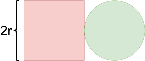
The Monte-Carlo approach starts with a random sample \((x_i, y_i)\) in a square of size \(2r \times 2r\), then it is tested against the following inequality:
\[r > \sqrt{x_i^2 + y_i^2},\]and labelled as belonging to inside (green) or outside (red) the circle if the inequality holds or not, respectively.
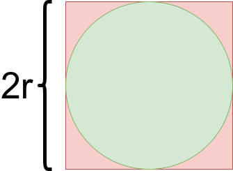
To estimate the value of \(\pi\), the number of points inside the circle (green) are counted and their ratio against total points sampled (green + red) is calculated to get an estimate of \(\pi\) as:
\[\frac{green\_pts}{green\_pts + red\_pts} = \frac{Area\_of\_circle}{Area\_of\_square} = \frac{\pi}{4}\]
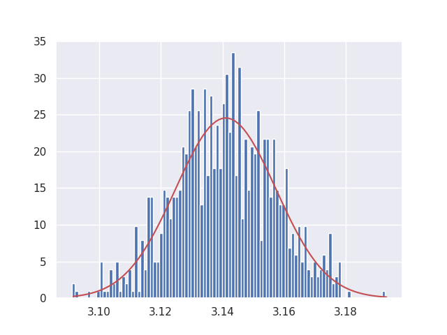
As with any process, the sampling process in Monte-Carlo estimation is noisy. If we can sample infinite number of points, then we will reach to an accurate estimated \(\pi\). However, in reality we can only sample a finite set of points and hence can achieve an estimate that is noisy due to the random sampling. However, if we repeat the experiment a number of times - we get many noisy estimates of \(\pi\). Looking at their distribution, we can notice that the predictions follow Gaussian distribution.
Relation to data-driven machine learning
Similar to our example of Monte-Carlo based estimation of the true value of \(\pi\), modern data-driven machine learning methods use a finite amount of random samples (data collected independently) to build a model of the underlying reality. Since we cannot have infinite amount of data available and the data collection/labelling process can be noisy, there are obvious errors/noise in the model which interestingly follow a Gaussian distribution due to the central limit theorem. As an example, this is one of the reason why ensemble-based learning, where outputs from multiple models are aggregated, are able to show less error in their predictions. Aggregation of outputs across an ensemble has its root in the central limit theorem and, hence, directly relates to the errors following a Gaussian distribution.
Looking at the above examples, we can relate the use of Gaussian distributions as the building blocks for data-driven models that can see beyond the variations/noise resulting from limited sampling of the world. In what follows, I plan to explore this and introduce basic learning methods utilising Gaussians that can enable us to achieve better data-driven models.