This post is aimed at implementing and showing some interesting use cases for Class Activation Maps (CAMs) using its description from the original paper “Learning Deep Features for Discriminative Localization”. For this, I will be using PyTorch to implement the method to get CAMs out of relevant deep learning classification models.

More specifically this post will cover:

• What are Class Activation Maps (CAMs)? How are they useful?
• How to implement an approach to get CAMs from a PyTorch model?
• Applications of CAMs in terms of getting more information out of classification models.

This post is based on previously proposed ideas and implementations, I only attempt to implement the equations from the above-mentioned paper and have certainly got the inspiration for the implementation and a lot of help in understanding the ideas from the following previous works:

• This blog post and accompanying code for implementing CAMs using PyTorch. Although I take a different approach as compared to this for getting the CAMs, the post-processing is directly taken from this implementation.
• Inspired by London PyTorch meetup talk given by Misa Ogura about FlashTorch, which provides a number of feature visualisation methods built on top of PyTorch.
• A number of CAMs-based papers, in particular I found this, this and this paper extremely useful for understanding the method.
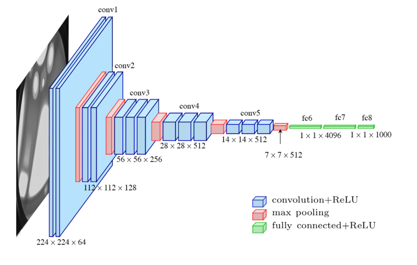
• Illustration of VGG network from https://tsapps.nist.gov/publication/get_pdf.cfm?pub_id=924455

What are Class Activation Maps (CAMs)?

Deep neural networks that are trained to address image classification tasks, consist of several layers (including convolution, pooling, activation, dense etc) that are applied to the image to infer the object class present in a given image. Image classification models extracts ‘what’ rather than ‘where’ the object is. This is often achieved through repeatedly applying pooling operations to loose the location and extract the object class information from image features. For example, a VGG architecture applies MaxPooling operations after each convolution to extract relevant features (as shown in Figure below).

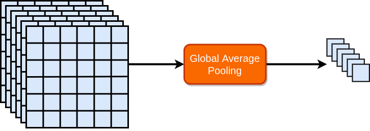
One such pooling operation that appears in state-of-the-art classification methods is called global average pooling (GAP) which takes average of all spatial locations in a given feature map (as depicted in Figure below).

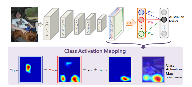
In networks where GAP appears just before the last dense layer (e.g. resnet, densenet, squeezenet), the method from “Learning Deep Features for Discriminative Localization” proposes to provide class activation maps by preserving the featuremaps before GAP and applying class weights from the following dense layer. This concept is captured in the Figure 2 of the paper, a copy of which appears below:

To define the CAMs mathematically, let \(f(x, y, c)\) be the output activation of the last layer before the global average pool layer, where x and y are indices for spatial locations and c are channels. Applying global average pooling gives:

where \(\|XY\|\) is the spatial size of \(f\).

After global pooling \(f_g(c)\) is fed into final dense layer which applies weights \(w(c, k)\) to give final prediction \(y\) as:

To get CAMs, the authors propose to remove the global average pool layer and directly apply weights for the predicted class \(j\) as:

How are CAMs useful?

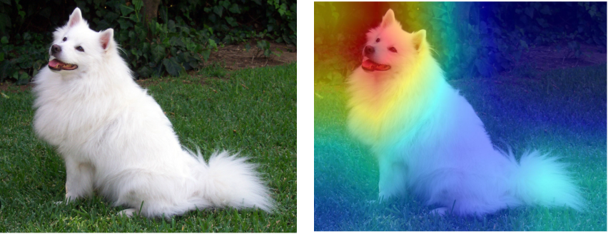
CAMs can be quite useful in understanding what a classifier is seeing in making the decision. For example, for the following image of a dog CAM indicates that the decision being made is based on the facial features of the dog, which does make sense as that is primarily what differentiate it from other animals.

Implementing CAMs in PyTorch

As outlined in this blog post and accompanying code one way to get Class Activation Maps is by extracting the relevant activation before global average pool layer and using it in weighted sum equation for the predicted class. There are two main issues with this approach, 1) it leads to significant manual work in identifying and fetching the relevant tensor and 2) for each output class the weighted sum needs to be repeated.

I attempt to address these issues by implementing CAMs in a slightly different way. Given a neural network with a global average pool layer at the second last layer as shown in fgure below:

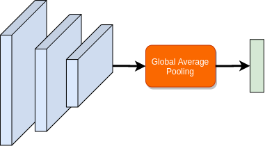
I replace the global average pool with a custom reshape layer, such that it reshapes the tensor to utilise the following dense layer for computing weighted sum of the activation map (as can be seen below). This operation reshapes \(f\) to have shape \(f(c, x\times y)\), meaning it collapses spatial dimension into a single dimension, while permutes to make channel dimension as the first dimension. This means when we apply the following dense layer. i.e. \(w \cdot f\), we directly calculate CAMs for each class in the output \(y(j, x \times y)\). After prediction, \(y\) can be reshaped to restore the spatial dimensions and visualise the CAMs. My current implementation for this is limited to batch size of 1 input as well as to only the networks that use global average pool layer as the second last layer in the network.

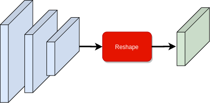
I implement the above using PyTorch to have a custom reshape layer as torch.nn.Module module:

class ReshapeModule(torch.nn.Module):
    def __init__(self):
        super(ReshapeModule, self).__init__()

    def forward(self, x):
        b, c, h, w = x.shape
        x = x.view(b*c, h*w).permute(1, 0)
        return x

Notice that the reshape layer uses tensor.view() to first reshape the featuremap to collapse the spatial dimensions into one. It then permutes channels with this dimension, such that the next dense layer can operate on each channel to give an output with spatial dimensions.

Next, in order to find the relevant global average pool layer and replace with my custom reshape layer I implement the following function which searches for the relevant global average pool layer within the network and replaces it with a custom reshape layer:

def modify_model_cam(model):
    """Modifies a pytorch model object to remove last 
    global average pool and replaces with a custom reshape
    module that enables generating class activation maps as 
    forward pass
    Args:
        model: pytorch model graph
    Raises:
        ValueError: if no global average pool layer is found
    Returns:
        model: modified model with last global average pooling 
                replaced with custom reshape module
    """

    # fetch all layers + globalavgpoollayers
    alllayers = [n for n, m in model.named_modules()]
    globalavgpoollayers = [n for n, m in model.named_modules(
    ) if isinstance(m, torch.nn.AdaptiveAvgPool2d)]
    if globalavgpoollayers == []:
        raise ValueError('Model does not have a Global
                            Average Pool layer')

    # check if last globalavgpool is second last layer - 
    #   otherwise the method wont work
    assert alllayers.index(globalavgpoollayers[-1]) == len(
        alllayers)-2, 'Global Average Pool is not second last layer'

    # remove last globalavgpool with our custom reshape module
    model._modules[globalavgpoollayers[-1]] = ReshapeModule()

    return model

Finally, given an image and our modified model, I use the following inference function to directly get CAMs as output of the modified network as well as compute class prediction probabilities from CAMs:

def infer_with_cam_model(cam_model, image):
    """Run forward pass with image tensor and get class activation maps
    as well as predicted class index
    Args:
        cam_model: pytorch model graph with custom reshape module
         modified using modify_model_cam()
        image: torch.tensor image with preprocessing applied
    Returns:
        class activation maps and most probable class index 
    """
    with torch.no_grad():
        output_cam_acti = cam_model(image)

        _, output_cam_idx = torch.topk(torch.mean(
            output_cam_acti, dim=0), k=10, dim=-1)

    return output_cam_acti, output_cam_idx

Application of CAMs in getting more information out of classification models

Class Activation Maps can be quite useful in understanding the regions of interest in a given image that are used by the model to give the corresponding class prediction. As is apparent, such visualisation helps in debugging and building further understanding on whether a model has learned meaningful representations.

In addition to the above, CAMs may also be useful in the following two scenarios:

Object localisation

As discussed in this paper, CAMs can be useful to localise relevant features for a given object. Specifically this is useful when there exist multiple objects in the image, where the classifier may be confused but still able to give high probability for each class in the image. We can use each of those confusion classes along with CAMs to visualise where each object is in the image (an example of such case appears in the Figure below).

Detecting lesions in medical images

As described in this paper, CAMs may be quite useful for medical imaging problems where the end goal is to detect lesions. Using CAMs this can be achieved with only classification labels to train a classifier.

Below is an example from a pneumonia classifier trained using this dataset from kaggle. The example shown is of a patient with pneumonia, where the image regions that are useful for making the decision about pneumonia classification are highlighted using CAMs:

All code accompanying this post can be accessed at: https://github.com/adeeplearner/ClassActivationMaps