In the previous post, I went through some areas where a Gaussian distribution could be useful. This post is going to be focused on implementation of Gaussians. Specifically, we will be implementing our first Gaussian, its discrete integral approximation and different comparison metrics that can be used to compare two distributions. I will be using Python’s NumPy library for all numerical operations in this post.

The content of this post is based on the following Wikipedia pages:

• https://en.wikipedia.org/wiki/Normal_distribution
• https://en.wikipedia.org/wiki/Bhattacharyya_distance
• https://en.wikipedia.org/wiki/Kullback%E2%80%93Leibler_divergence
• https://en.wikipedia.org/wiki/Entropy_(information_theory)

All implementations are my own and can be accessed as a single script at: https://github.com/adeeplearner/Part2-Gaussians

Implementing our first Gaussian function

Recall from the previous post that a one-dimensional Gaussian is defined as:

We use Python’s NumPy library to implement this one-dimensional Gaussian as follows:

import numpy as np

def Gaussian1D(x, mu, sigma):
    """Implements 1D Gaussian using the following equation
     G(x) = \frac{1}{\sigma\sqrt{2\pi}} 
              e^{-\frac{1}{2}[\frac{(x-\mu)^2}{\sigma^2}]},
    Args:
        x (np.array): x points to evaluate Gaussian on 
        mu (float): mean of the distribution
        sigma (float): standard deviation of the distribution

    Returns:
        np.array: distribution evaluated on x points
    """
    ATerm = 1/(sigma * np.sqrt(2 * np.pi))
    BTerm = np.exp(-0.5 * ((x-mu)/sigma) ** 2)
    return ATerm * BTerm

In the function Gaussian1D(x, mu, sigma), x correspond to \(x\) values for which the function is evaluated, and mu and sigma correspond to \(\mu\) and \(\sigma\), respectively.

The function \(g(x)\) in our equation is defined over a continuous space, however for most machine learning related tasks we are limited by modern computers to resort to discrete evaluation of the function (unless there exists an analytic solution). In our first implementation using NumPy, we evaluate our function on discrete x values. To achieve this, we define a grid of x-axis values using NumPy’s linspace function and evaluate a Gaussian with \(\mu=0\) and \(\sigma=1\) as follows:

x_grid = np.linspace(-6, 6, 100)
y = Gaussian1D(x_grid, mu=0, sigma=1)

We can now proceed to visualise our first Gaussian using Maplotlib:

import matplotlib.pyplot as plt

plt.figure()
ax = plt.gca()
plt.plot(x_grid, y)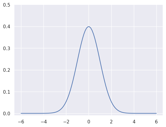

In the next section, I will go over some interesting properties and further build on our example to provide tools for comparing two Gaussians.

Properties of probability density functions (PDF)

The Gaussian function is a probability density function (PDF), defined over a continuous random variable (in our one-dimensional case \(x\)) that provides a likelihood of the random variable being within a specific range.

Mathematically a PDF function \(P(x)\) is any function that satisfies the following properties:

• For any interval \([a, b]\), the probability can be found as \(P( a \lt x \lt b) = \int_{a}^{b} P(x) dx\). This also corresponds to calculating the area under the curve for a discrete distribution.
• The value of the function \(P(x)\) at any point is always non-negative, i.e. \(P(x) \ge 0 \,\,\, \forall x\).
• As area under the curve/integral corresponds to probability over a range of \(x\), therefore probability taken over all possible values of \(x\) should be \(1\). Hence, \(\int_{-\infty}^{+\infty} P(x)dx = 1\)

In case of our Gaussian function, the area under the curve defines the corresponding probability of \(x\) for the given range. As we have to resort to discrete evaluation of the function, therefore we can approximate the integral as area under the curve defined by:

where \(\delta x\) is the step size in discrete values of x. As we will see later in this post, integrals play an important role when measuring similarity between two distributions, and hence can be used to define probabilistic objective functions in machine learning.

Implementing discrete integral for Gaussians

We can implement a discrete integral approximation for our Gaussian example. As indicated in previous section this can be approximated using equation \(\sum P(x) \delta x\), which we implement in NumPy as follows:

def discreteIntegral1D(p, dx):
    """Implements 1D discrete integral using the following equation
    integral \approx \sum_x P(x) dx

    It can also be thought of as area under the curve

    Args:
        p (np.array): points in distribution
        dx (float): delta x, spacing of discrete x points

    Returns:
        float: integral over the discrete space
    """
    return np.sum(p) * dx

We can use the integral to extend our example Gaussian evaluation to also compute the integral of our Gaussian.

x_grid = np.linspace(-6, 6, 100)
y = Gaussian1D(x_grid, mu=0, sigma=1)
deltax = x_grid[1]-x_grid[0]
integral = discreteIntegral1D(y, deltax)
print('Integral is: %f' % integral)
# Output:
# Integral is: 1.000000

The figure below visualises this integral in discrete space achieved through area under the curve.

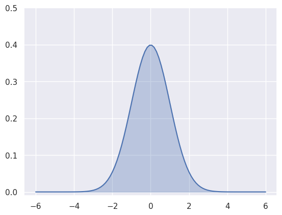
Estimating the integral for a given range gives us probability of \(x\) taking values within that range. We can extend our example to evaluate integral within \(\pm 1\) range as follows:

x_grid = np.linspace(-6, 6, 100)
x_grid_sel = x_grid[np.where(np.logical_and(x_grid>=-1, x_grid<=1))[0]]
y_sel = Gaussian1D(x_grid_sel, 0, 1)

prob = discreteIntegral1D(y_sel, x_grid_sel[1]-x_grid_sel[0])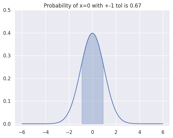

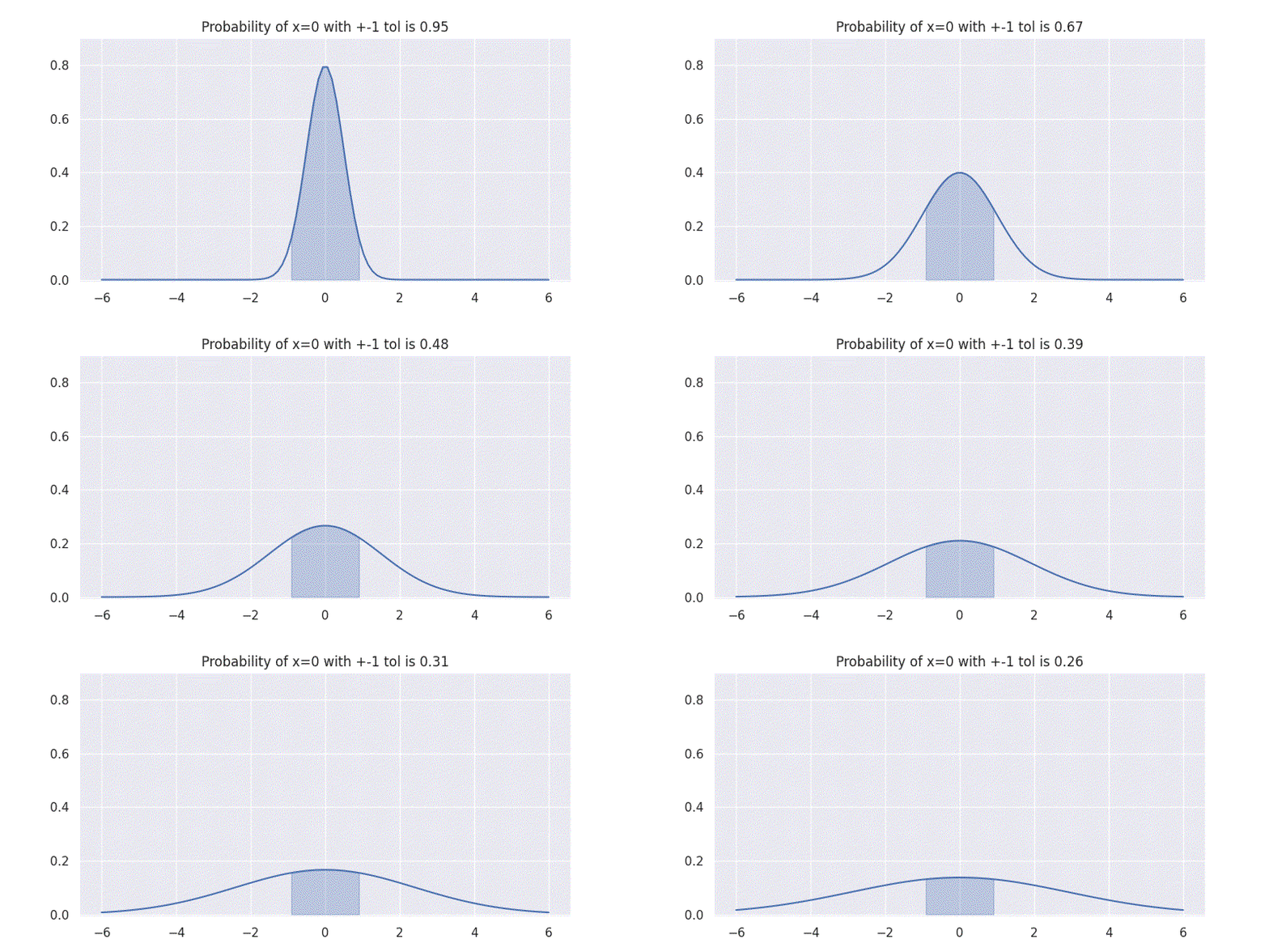
One interesting aspect to understand here is that the standard deviation \(\sigma\) controls the spread of our distribution. It is also directly related to the confidence our distribution has on the mean \(\mu\) prediction. This can be seen by evaluating our above integral within \(\pm 1\) range while varying \(\sigma\) as shown in figure below:

Comparing two Gaussians

In modern machine learning methods, especially deep neural networks, we often look at a loss function that compares the model’s predictions against groundtruth labels and provides a measure of ‘loss’. It is, therefore, relevant to understand the comparison metrics when directly learning probability distributions. In this section I introduce and implement two widely used measures that are used for comparing two Gaussians. In a later blog post, I plan to revisit these and show how they can be directly used in a simple optimisation algorithm to learn the groundtruth distributions.

Let \(P(x)\) and \(Q(x)\) be two distributions, the two most widely used methods for comparing \(P(x)\) and \(Q(x)\) are defined as follows:

Bhattacharyya distance

Bhattacharyya distance measures the similarity of two probability distributions. It is defined as:

As can be seen, the main idea of this metric is to measure the overlap between the two distributions. \(\sqrt{\cdot}\) normalises the distance so the term \(\sqrt{P(x)Q(x)}\) is in the range \([0, 1]\). For the case where \(P(x) = Q(x)\), i.e. two distributions are same, this term is equal to \(0\).

For our discrete approximation, the above equation can be rewritten as:

We can implement Bhattacharyya distance between two discrete distributions using our discreteIntegral1D() function as follows:

def bhattacharyyaDistance(p, q, dx):
    """Implements Bhattacharrya Distance between 
    two distribution P(x) and Q(x)
    
    Uses the following equation:
    D_{BC}(P, Q) \approx -\log \sum_x \sqrt {P(x) Q(x)} dx

    Details about Bhattacharyya distance:
    https://en.wikipedia.org/wiki/Bhattacharyya_distance

    Args:
        p (np.array): P(x) discrete distribution 
        q (np.array): Q(x) discrete distribution
        dx (float): delta x, spacing of discrete x points

    Returns:
        float: Bhattacharyya distance
    """
    return -np.log( discreteIntegral1D( np.sqrt(p*q), dx ) )

Kullback-Leibler Divergence

Kullback-Leibler divergence measures how different a given distribution \(Q(x)\) is from a reference distribution \(P(x)\). It is defined as:

KL divergence has its roots in information theory, which why it is sometimes referred to as relative entropy. We can see why this is the case by expanding the divergence equation as:

Notice that the term \(T1\) corresponds to Shannon’s entropy, whereas term \(T2\) is relative entropy term comparing the two distributions. In machine learning, \(P(x)\) is the groudtruth distribution which does not change during training and hence \(T1\) remains constant. Learning \(P(x)\) through \(Q(x)\) only requires minimising \(T2\).

For our discrete case, we can get the following equation for KL divergence:

Similar to our previous code, we can also implement KL divergence using our discreteIntegral1D() function as follows:

def kullbackLeiblerDivergence(p, q, dx):
    """Implements Kullback-Leibler Divergence between 
    two distribution P(x) and Q(x)
    
    Uses the following equation:
    D_{KL}(P \parallel Q) \approx \sum_x P(x) \log (\frac{P(x)}{Q(x)}) dx

    Details about KL divergence:
    https://en.wikipedia.org/wiki/Kullback%E2%80%93Leibler_divergence

    Args:
        p (np.array): P(x) discrete distribution 
        q (np.array): Q(x) discrete distribution
        dx (float): delta x, spacing of discrete x points

    Returns:
        float: Kullback-Leibler Divergence
    """
    return discreteIntegral1D( (p * np.log(p/q)), dx )

Comparing two Gaussians: We have now all the tools to check how two Gaussians differ from each other. So lets get to coding two Gaussians and comparing them using the two metrics defined about:

x_grid = np.linspace(-6, 6, 100)

P_gt = Gaussian1D(x_grid, mu=0, sigma=1)
P_m = Gaussian1D(x_grid, mu=3, sigma=1)

deltax = x_grid[1]-x_grid[0]

kldiv = kullbackLeiblerDivergence(P_gt, P_gt, deltax)
bc = bhattacharyyaDistance(P_gt, P_gt, deltax)

print('Comparing same distributions')
print('KL div is: %f' % kldiv)
print('BC is: %f' % bc)

print('')
kldiv = kullbackLeiblerDivergence(P_gt, P_m, deltax)
bc = bhattacharyyaDistance(P_gt, P_m, deltax)
print('Comparing different distributions')
print('KL div is: %f' % kldiv)
print('BC is: %f' % bc)

# Output: 
# Comparing same distributions
# KL div is: 0.000000
# BC is: 0.000000

# Comparing different distributions
# KL div is: 4.500000
# BC is: 1.125003

We can also sweep through different mean and standard deviation for model distribution \(Q(x)\) and report our metrics in a nice plot:

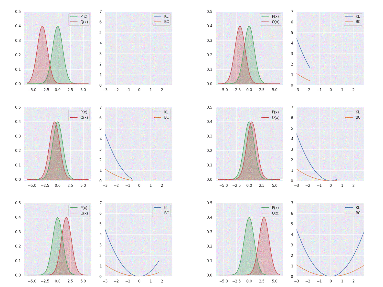
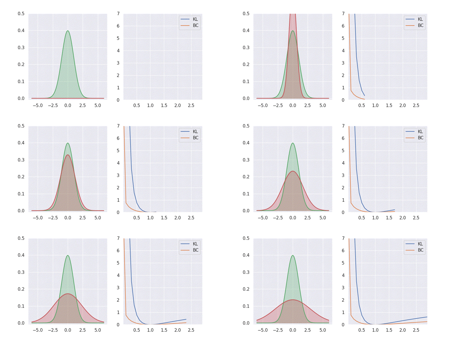
Notice in the above plot the error in the KL divergence looks similar to a quadratic curve (especially when varying mean of \(Q(x)\)). This is because the KL divergence forms the basis for both cross-entropy loss and mean-square error(MSE/L2) loss functions which are widely deployed for addressing classification and regression problems, respectively. As I explored in an earlier blog post, using KL divergence for learning Gaussian distribution is where we get mean squared error (aka L2 loss).

In the following blog post we will build upon our implementation of the comparison metrics to understand how they can be used for learning a target Gaussian distribution.