Until now, I have discussed what Gaussians are? how can we implement them? and how different metrics can be defined to compare two Gaussian distributions? This brief post is going to go into detail of how we can enable a neural network to learn to output Gaussian distributions.

More precisely this post will cover:

• The concept of a loss function and its minimisation.
• How to take partial derivatives of a loss function?
• How to learn a simple neural network that outputs Gaussian distributions?
• Incorporating the above into much bigger neural networks

The content of this post is largely based on Andrew Ng’s excellent Deep Learning Specialization course. To learn Gaussians, a simple derivation is used, which can be worked out as a quick loss derivation exercise and follows directly from my previous posts on the same topic.

I have written the following two pieces of code to demonstrate the examples in this post:

https://github.com/adeeplearner/ParabolaGradient

https://github.com/adeeplearner/KLDivLossForGaussians

What is a loss function?

Imagine you are at the top of a hill, wanting to hike down into a freshwater lake in the nearby valley. Since you are high-up, you can see down the hill and work out the easiest path to get down. Along the way, you end up making some adjustments to keep the path as simple as possible but still aiming to get down to the lake. After a bit of work, you finally manage to reach the lake and enjoy the freshwater from it.

Congratulations! You have just implemented your very own loss function and its optimisation without even realising it. In our example above, your objective was to get to the lake. This is what you were always trying to solve. In neural networks, a loss function can be thought of a similar objective. Once this objective is defined we can start optimising with small steps (just like the steps/path you took to get to the lake) to make our model get to the final solution. Similar to our example, optimising a loss function may mean that we want to minimise its output, which in our example was our altitude.

What are partial derivatives? How to get them for a given function?

Before we dive into optimising a loss function, lets first take a quick refresher about partial derivatives as these are essential when using a loss function to learn a neural network. The example below is taken from partial derivatives wikipedia page. I have tried to simplify it and provide some context with respect to neural networks.

A partial derivative is a derivative of a function of more than one variables, with respect to one of the variable. Suppose you have the following function \(f(x, y)\):

Then the partial derivative of \(f\) with respect to \(x\) is defined as:

Here the symbol \(\partial\) differentiates the above from a derivative, indicating the presence of more than one variable. In a similar manner, you can also work out the partial derivative of \(f\) with respect to \(y\):

One important point here is that for partial derivatives to be worked out, the function \(f\) needs to be fully differentiable. This is the reason why in neural networks literature differentiability of a given function is a big deal as it means we can use it within an existing optimisation framework.

Why take partial derivatives?

So you may be wondering, whats the big deal with partial derivatives? Why do we take these in the first place? The example in the above equations is for a simple parabola function. The landscape of this function looks something like as follows:

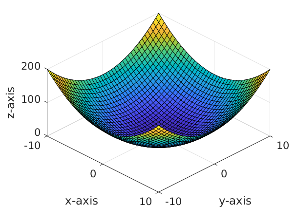
Now if we start with a random point \((x, y)\) and optimise to find minima of function \(f\), we would be trying to find the direction to move our initial point \((x, y)\) to, such that it minimises the value of \(f(x, y)\). Here partial derivatives come into play, which provides us with the direction in which the function increases with respect to each variable. In order to minimise \(f\), all we have to do is move our initial guess in the opposite direction (negative gradient) to these derivatives. This can be achieved for our simple example as:

The optimisation method described with reference to the above two equations is referred to as gradient descent, where we descent our loss landscape using gradients. \(\alpha\) in the above equation is the learning rate, which determines how big each step in our optimisation would be.

If we try to visualise the gradient descent optimisation, it looks quite similar to our initial hill descent example:

Note that the animation above also includes momentum term within gradient descent, which enables our optimisation to have inertia resulting in motion that looks like a ball rolling down the loss landscape.

Code for the above example is accessible at: https://github.com/adeeplearner/ParabolaGradient

Loss function for learning a Gaussian distribution

Now that we know how to define a loss function and use a simple gradient descent optimisation on it, we can start looking into how a loss function can be defined to get neural networks to output Gaussian distributions.

Recall from this previous post that given a ground truth distribution \(P_{gt}\) and a model distribution \(P_{m}\), where both \(P_{gt}\) and \(P_{m}\) are Gaussians distributions, a loss metric between the two can be defined as:

In the above function, \(\mu_{gt}\) and \(\sigma_{gt}\) are parameters of our ground truth Gaussian distribution, which are usually fixed during optimisation. Whereas \(\mu_{m}\) and \(\sigma_{m}\) are parameters of our model distribution that are learned during optimisation. Minimising function \(D_{kl}\) results in finding the parameters \(\mu_{m}\) and \(\sigma_{m}\) that approach the value of \(\mu_{gt}\) and \(\sigma_{gt}\).

In the subsequent sections, we will use the above equation as our loss function to enable a neural network to learn a Gaussian distribution.

Partial derivatives of \(D_{kl}\)

We can take partial derivates of \(D_{kl}\) with respect to each variable \(\mu_{m}\) and \(\sigma_{m}\) as:

and,

These can be used in the optimisation algorithm, such as gradient descent to enable learning the model distribution \(P_{m}\) as the output of a neural network.

Implementing our loss using NumPy

We can implement the loss function and its partial derivatives using NumPy. In order to keep things in one place, we make use of python class and define a forward function, which calculates the value of \(D_{kl}\), and a backward function which computes the gradients \(\frac{\partial D_{kl}}{\partial \mu_{m}}\) and \(\frac{\partial D_{kl}}{\partial \sigma_{m}}\).

Here is how the code looks for this:

class KLDivUnimodalGaussianLoss:
    def forward(self, target, output):
        """
        Implements
        
        D_{KL}(P_{gt} \parallel P_{m}) = -\frac{1}{2} + \log \big(\frac{\sigma_{m}}{\sigma_{gt}}\big) + \frac{1}{2 \sigma_{m}^{2}} \big[ \sigma_{gt}^2 + (\mu_{gt}-\mu_{m})^2 \big]
        """

        return -0.5 + np.log(output[:, 1]/target[:, 1]) + (1/(2*(output[:, 1]**2))) * (target[:, 1]**2 + (target[:, 0] - output[:, 0])**2)
    

    def backward(self, target, output, grad_output):
        """
        Implements

        \partial D_KL/\partial \mu_m
        and
        \partial D_KL/\partial \sigma_m
        
        """
        deloutput = np.zeros_like(output)
        
        # \partial \mu
        deloutput[:, 0] = (output[:, 0] - target[:, 0])/(output[:, 1]**2)
        # \partial \sigma
        deloutput[:, 1] = 1/output[:, 1] - (1/output[:, 1]**3)*(target[:, 1]**2 + (target[:, 0]-output[:, 0])**2)

        return None, deloutput * grad_output

Simple network for testing

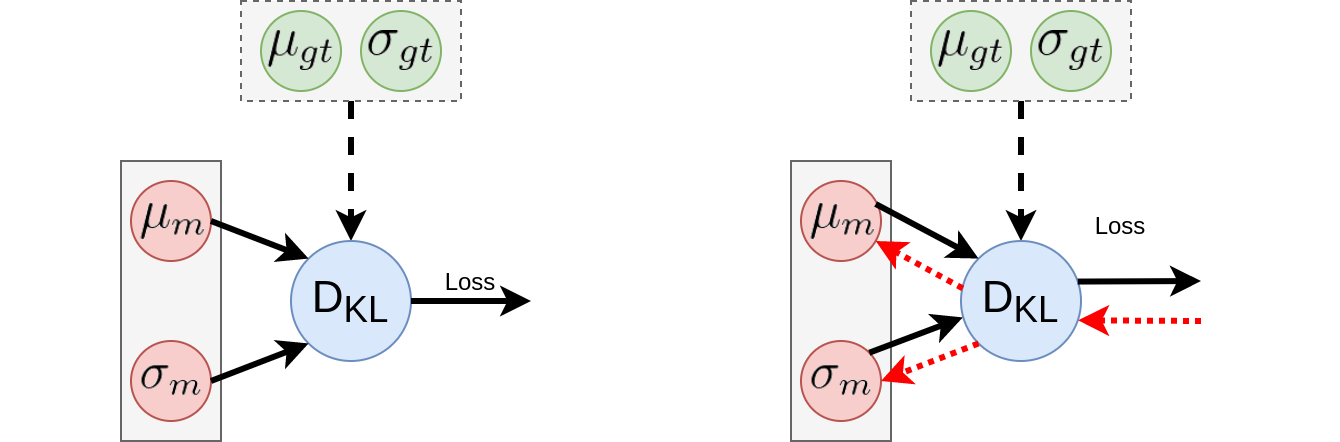
Now that we have our loss function, we define a simple network to use for testing whether it works as expected. In order to do this, we initialise two nodes with variable \(\mu_{m}\) and \(\sigma_{m}\). We can then use our loss function, along with ground truth \(\mu_{gt}\) and \(\sigma_{gt}\), to compute the loss in the forward pass. In the backward pass, we can propagate gradients from our loss function and use them to optimise \(\mu_{m}\) and \(\sigma_{m}\). This makes a small network with forward and backward pass as shown below:

Finally, we can consolidate everything into a simple gradient descent optimisation using the equations:

The above optimisation can be implemented into an optimisation function as follows:

def optimise_gradient_descent(param_p, param_q, x_grid=np.linspace(-6, 6, 100), lr=0.01, save_interval=None, n_epochs=1000000):
    param_q_list = []
    loss_list = []

    # keep record of loss, to check termination
    loss_stack = deque(100*[0], 1000)

    kl = KLDivUnimodalGaussianLoss()

    for epoch in range(n_epochs):
        print('%d/%d' % (epoch, n_epochs))

        # do forward pass to calculate loss
        out = kl.forward(param_p, param_q)
        loss_stack.append(out[0])

        avg_loss = sum(loss_stack)/len(loss_stack)
        
        if avg_loss < 0.000000001:
            break
        
        # do backward pass to optimise params
        delout = kl.backward(param_p, param_q, 1)[1] 
        param_q = param_q - lr * delout
    
        if save_interval != None and epoch % save_interval == 0:
            param_q_list.append(param_q)
            loss_list.append(out[0])

    return param_q, param_q_list, loss_list

If all goes well, our optimisation should result in \(\mu_{m} = \mu_{gt}\) and \(\sigma_{m} = \sigma_{gt}\), confirming that everything works as expected. Below animation shows minimisation of \(D_{kl}\) along with how the two Gaussians adjust during optimisation.

Code for the above example is accessible at: https://github.com/adeeplearner/KLDivLossForGaussians

Applying our loss to bigger neural networks

Now that we know that our loss function works as expected, we can go ahead and incorporate it into bigger neural networks. This can be achieved by converting the variables \(\mu_{m}\) and \(\sigma_{m}\) in our simple example to be two neurons and connecting them to the output of a neural network. This network should look like as follows:

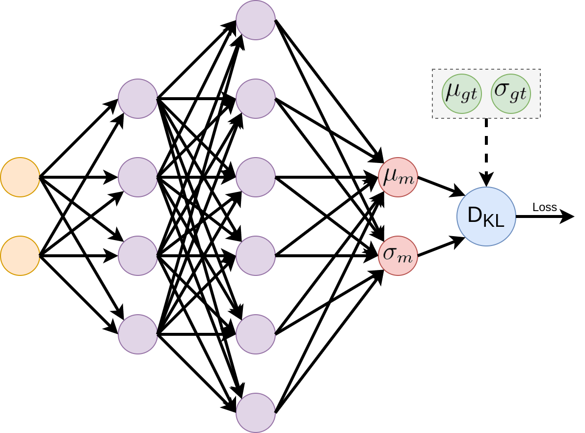
With the above modifications, the gradients coming from our loss to \(\mu_{m}\) and \(\sigma_{m}\) will be backpropagated into the network using the chain rule. These would then be applied to update parameters at each neuron in the network, such that the network learns to output \(\mu_{m}\) and \(\sigma_{m}\) as close to ground truth as possible.

Next step would be to apply our loss and network to learn from a dataset. However, in the interest of the length of this post, I will leave this step for another post.